BOLFI 🔗
“Bayesian Optimization for Likelihood-Free Inference of Simulator-Based Statistical Models” (2016) by Michael U. Gutmann and Jukka Corander.
 Available as 🔗 presentation slides or as a 🔗 blogpost.
Problem 🔗
- Topic: Statistical inference for models where:
- The likelihood \(p_{\mathbf{y}|\mathbf{\theta}}\) is intractable 🔮 (e.g. analytical form is unknown/costly to compute).
- \(\implies\) inference with likelihood \(\mathcal{L}(\mathbf{\theta}) = p_{\mathbf{y}|\mathbf{\theta}}(\mathbf{y}_o | \mathbf{\theta})\) is not possible.
- Simulating data 🤖 from the model is possible.
- Using a simulator-based statistical model (implicit/generative model), i.e. a family of pdfs \(\left\{p_{\mathbf{y} \mid \mathbf{\theta}} \right\}_{\mathbf{\theta}}\) of unknown analytical form which allows for exact sampling of data \(\mathbf{y} \sim p(\mathbf{y}|\mathbf{\theta})\)
- The likelihood \(p_{\mathbf{y}|\mathbf{\theta}}\) is intractable 🔮 (e.g. analytical form is unknown/costly to compute).
- Inference principle: Find parameter values \(\theta\) for which there is a small distance between
- the posterior of the simulated data \(\mathbf{y}\), and
- the observed data \(\mathbf{y}_o\).
Other assumptions 🔗
- Only a small number of parameters are of interest (theta is low-dimensional)
- Data generating process can be very complex
Existing methods 🔗
For likelihood-free inference with simulator-based models, the basic idea is to identify model parameters by finding values which yield simulated data that resemble the observed data.
- “Approximate Bayesian computation” (ABC), originated in genetics 🔬
- “Indirect inference”, originated in economics 📈
- “Synthetic likelihood”, originated in ecology 🌲
Conventional ABC 🔗
- “Bayesian forward modeling”, i.e. likelihood-free rejection sampling (LFRS)
- Let \(\mathbf{y}_o\) be the observed data. For many iterations:
- Sample \(\theta\) from proposal distribution \(q(\theta)\).
- Sample \(\mathbf{y}|\theta\) according to the data model.
- Compute distance \(d(\mathbf{y}, \mathbf{y}_o)\)
- Keep if \(d(\mathbf{y}, \mathbf{y}_o) \leq \epsilon\); discard otherwise.
- Different \(q(\theta)\) for different algorithms
- If \(\epsilon\) is small enough, kept samples are samples from an approximate posterior
Implicit likelihood approximation 🔗
There is an implicit likelihood approximation going on here.
- Compute likelihood (probability of generating data like \(\mathbf{y}_o\) given hypothesis \(\theta\)) empirically
- Proportion of kept (green) samples
- \(L(\theta) \approx \frac{1}{N} \sum_{i=1}^{N} \mathbb{1}\left(d\left(y_{o}^{(i)}, y^{\circ}\right) \leq \epsilon\right)\)
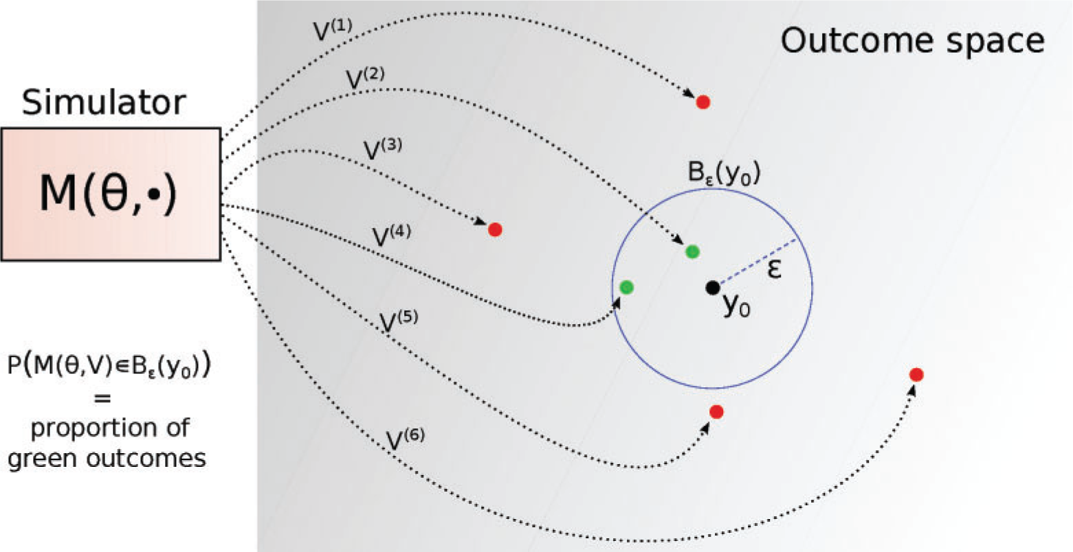
Illustration of rejection sampling (Lintusaari et al., 2016)
Downsides 🔗
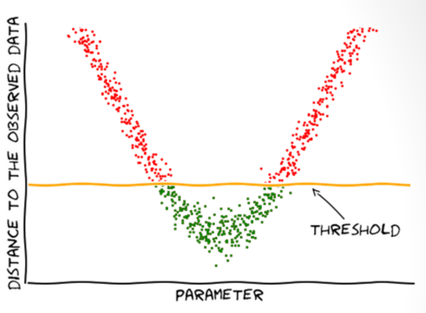
Inefficiencies of rejection sampling (Florent Leclercq, 2018)
\(L(\theta) \approx \frac{1}{N} \sum_{i=1}^{N} \mathbb{1}\left(d\left(y_{o}^{(i)}, y^{\circ}\right) \leq \epsilon\right)\)
- Rejects most samples when \(\epsilon\) is small
Does not make assumptions about the shape of \(L(\theta)\)
- Dependency of L on \(\theta\) is via the parameter used to generate theta, if we moved the threshold by just a little bit we don’t constrain the likelihood to be similar at all; no constraint on likelihood’s smoothness at all. Algorithm is given a lot of freedom but it becomes expensive. A lot of dependency on theta, as opposed to depending on say smoothness constraint.
Does not use all information available.
- You could, say, stop early after many rejections and conclude that the likelihood is low with high certainty.
Aims at equal accuracy for all parameters
- Computational effort \(N\) doesn’t depend on \(\theta\)
- E.g. prioritise for modal area
BOLFI 🔗
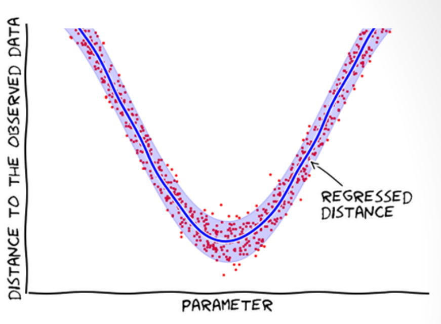
Advantages of BOLFI (Florent Leclercq, 2018)
- Does not reject samples; learns from them (i.e. builds a statistical model of the distances w.r.t. the parameters).
- Models the distances, assuming the average distance is smooth.
- Use Bayes’ theorem to update the proposal of new points.
- Prioritize parameter regions with small distances.
Regressing effective likelihood 🔗
- Data are tuples \((\theta_i, d_i)\), where \(d_i = d(\mathbf{y}_\theta^{(i)}, \mathbf{y}_o)\)
- Model conditional distribution \(d \mid \theta\)
Approximate likelihood function for some choice of \(\epsilon\):
- Use the probability under that extimated model that the distance is smaller than \(\epsilon\).
- \(\hat{L}(\theta) \propto \hat{P}(d\leq \epsilon \mid \theta)\)
- Choice of \(\epsilon\) is delayed until the end, after the learning of the model.
Regressing effective likelihood 🔗
- Fit a log Gaussian process (GP) to regress how the parameters affect the distances and use Bayesian optimization.
- Squared exponential covariance function
- Log transform because distances are non-negative
- Approach is not restricted to GPs
Data acquisition 🔗
- Use Bayesian optimization to prioritize regions of \(\theta\) where \(d\) tends to be small.
- Sample \(\theta\) from an adaptively constructed proposal distribution, e.g. the lower confidence bound acquisition function.
- \(\mathcal{A}_{t}(\theta)=\underbrace{\mu_{t}(\theta)}_{\text {post mean }}-\sqrt{\underbrace{\eta_{t}^{2}}_{\text {weight }} \underbrace{v_t(\theta)}_{\text {post var }}}\), \(t\): no. of samples acquired
- “We used the simple heuristic that \(\theta_{t+1}\) is sampled from a Gaussian with diagonal covariance and mean equal to the minimizer of the acquisition function. The standard deviations were determined by finding the end-points of the interval where the acquisition function was within a certain (relative) tolerance.”
- Approach is not restricted to this acquisition function.
Bayesian optimization in action 🔗
An animation of Bayesian optimization (Florent Leclercq, 2018)
Close the loop 🔗
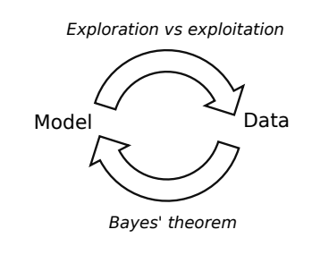
High-level mechanism of Bayesian optimization (Florent Leclercq, 2018)
- Exploration: where the uncertainty is high
- Exploitation: where posterior mean is smallest
- Use Bayes’ theorem to update the model in light of new data
- As opposed to usual applications of Bayesian optimization, here the objective function is highly stochastic.
Results 🔗
- Roughly equal results with 1000x fewer simulations
- Monte Carlo ABC: 4.5 days with 300 cores
- BOLFI: 90 minutes with seven cores
- Data of bacterial infections in child care centers.
- Data generating process is defined via a latent continuous-time Markov chain and an observation model.
- “Developed by Numminen et a.l (2013) to infer transmission dynamics of bacterial infections in day care centers.”
Figure 12 🔗
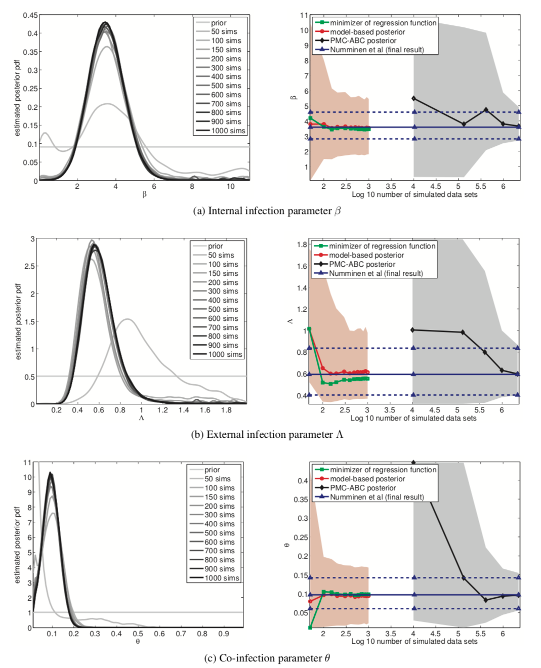
- Computational cost on log scale. 6 means a million; 3 means a thousand
- Blue line is reference for the inferred posterior mean at the very end of the standard PMC-ABC posterior method.
- Red line is the best, model-based posterior
- Confidence intervals are wider than conventional approach
Advantages 🔗
- Inference more efficient, far more comprehensive data analysis.
- Enables inference for e.g. models of evolution where simulating a single data set takes 12-24 hours.
- Enables investigation of model identifiability, or the influence of distance measure on likelihood function.
- We get an explicit construction of an approximate likelihood function, whereas with conventional ABC only had an implicit likelihood function.
Further research 🔗
- Distance measures
- Acquisition function
- Efficient high-dimensional inference
- Use this advantage from Bayesian optimization
Conclusion 🔗
BOLFI combines …
- Statistical modeling (GP regression) of the distance between observed and simulated data
- Decision making under uncertainty (Bayesian optimization).
…to increase efficiency of inference by several orders of magnitude.
Links and references 🔗
- Code: https://github.com/elfi-dev/elfi
- Demonstration: https://github.com/elfi-dev/notebooks/blob/master/BOLFI.ipynb
- Video: “Bayesian optimization for likelihood-free cosmological inference”
- Video: “Michael Gutmann: Bayesian Optimization for Likelihood-Free Inference - GPSS 2016”
Bibliography
Lintusaari, J., Gutmann, M. U., Dutta, R., Kaski, S., & Corander, J. (2016), Fundamentals and Recent Developments in Approximate Bayesian Computation, Systematic Biology. ↩
Leclercq, F. (2018). Bayesian optimisation for likelihood-free cosmological inference. Retrieved from http://www.florent-leclercq.eu/talks/2018-10-22_IHP.pdf. (Accessed on 11/03/2019. Recording at https://www.youtube.com/watch?v=orDbPZFd7Gk&t=41s.). ↩