Bayesian Meta-Learning
\(\text{“I can’t believe it’s not Bayesian”}\) \(\tiny \text{- Chelsea Finn, ICML 2019 meta-learning workshop}\)
Agenda
- Meta-learning: why, what, how?
- Bayesian meta-learning
- A few examples: fast and furious
- Bayesian model-agnostic meta-learning (MAML)
- Neural Process (NP)
- Deep meta-learning GPs
Why meta-learning?
- It is more human/animal-like 👪🐕: humans can learn from a rich ensemble of partially related tasks, extracting shared information from them and applying that on new tasks with few samples lake16_build_machin_that_learn_think_like_peopl
- Learning-to-learn has been studied in cognitive science lake15_human_level_concept_learning and psychology hospedales20_meta_learn_neural_networ,griffiths19_doing_more_with_less,
- It seeks to address data-hungry 💸 supervised deep learning.
- Data efficiency using prior knowledge transferred from related tasks.
- Successful applications in few-shot image recognition, data efficient reinforcement learning (RL), and neural architecture search (NAS).
- EfficientNet’s, current SoTA beating ResNet, are found via NAS.
What is meta-learning?
- Actually, you already know it—it’s a broad framework that encompasses a commonplace machine learning (ML) practice: hyperparameter search.
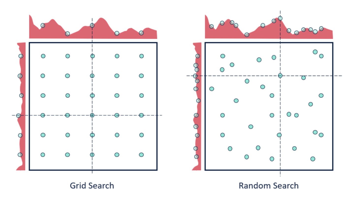
Figure 2: Hyperparameter searches (image source)
But really, what is it?
- Difficult to define, as it has been used in different ways, but a good start is:
The salient characteristic of contemporary neural-network meta-learning is an explicitly defined meta-level objective, and end-to-end optimization of the inner algorithm with respect to this objective hospedales20_meta_learn_neural_networ
Conventional vs meta-learning
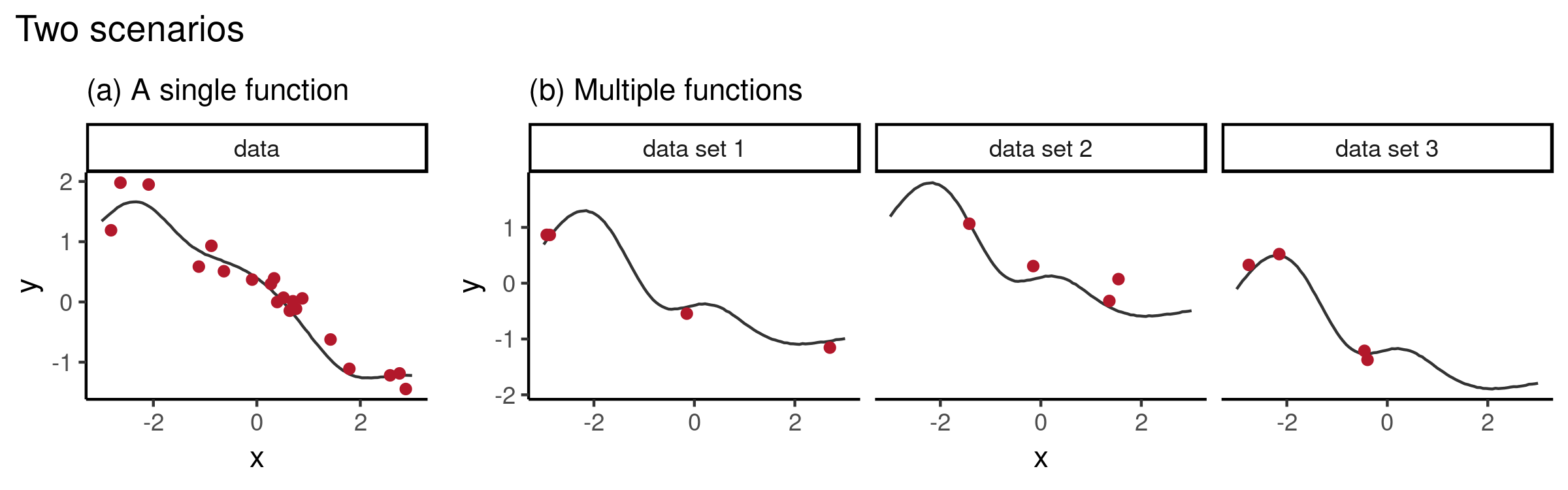
Figure 3: Conventional vs meta-learning for 1D function regression (image source)
- a): Single dataset \(\mathcal{D} = (x, y)_{i=1}^n, y_i = f_{\theta, \color{blue}{ \omega}}(x_i )\)
- Learn \(f_{\theta, \color{blue}{ \omega}}:\mathcal{X} \rightarrow \mathcal{Y}\) that is explicitly parameterized by \(\theta\) (e.g. neural network weights) and implicitly pre-specified by \(\color{blue}{\text{a fixed } \omega}\) (e.g. learning rate, optimizer).
- Optimize for \(\theta^* = \arg \min_\theta \mathcal{L}_\theta(\mathcal{D}; \theta, \color{blue}{\omega})\).
- b): Dataset of datasets \(\{\mathcal{D}_t \}_{t=1}^{3}\) from task distribution \(p(\mathcal{T}), \mathcal{T} = \{\mathcal{D}, \mathcal{L}\}\).
- Objective: \(\color{blue}{\text{A learnable }\omega}\) is optimized over \(p(\mathcal{T})\), i.e. \(\displaystyle \color{blue}{\omega^*} = \min _{\color{blue}{\omega}} \underset{\tau \sim p(\mathcal{T})}{\mathbb{E}} \mathcal{L}(\mathcal{D} ; \color{blue}{\omega})\).
- Meta-knowledge \(\color{blue}{\omega}\) specifies “how to learn” \(\theta\).
- E.g. Shared meta-knowledge \(\color{blue}{\omega}\) can encode the family of sine functions (everything but phase and amplitude) while \(\theta\) encodes the phase and amplitude.
Two phases of meta-learning methods
- Generally split into two phases hospedales20_meta_learn_neural_networ:
- Meta-training on \(\mathscr{D}_{\text {source}}=\left\{\left(\mathcal{D}_{\text {source}}^{\text {train}}, \mathcal{D}_{\text {source}}^{\text {val}}\right)^{(i)}\right\}_{i=1}^{M}\) entails \(\omega^{*}=\arg \max _{\omega} \log p\left(\omega | \mathscr{D}_{\text {source }}\right)\)
- Meta-testing (online adaptation) on \(\mathscr{D}_{\text {target}}=\left\{\left(\mathcal{D}_{\text {target}}^{\text {train}}, \mathcal{D}_{\text {target}}^{\text {test}}\right)^{(i)}\right\}_{i=1}^{Q}\) entails \(\theta^{*(i)}=\arg \max _{\theta} \log p\left(\theta | \omega^{*}, \mathcal{D}_{\text {target}}^{\text {train}}(i)\right)\). Evaluation done on \(\mathcal{D}_{\text {target}}^{\text {test}}\).
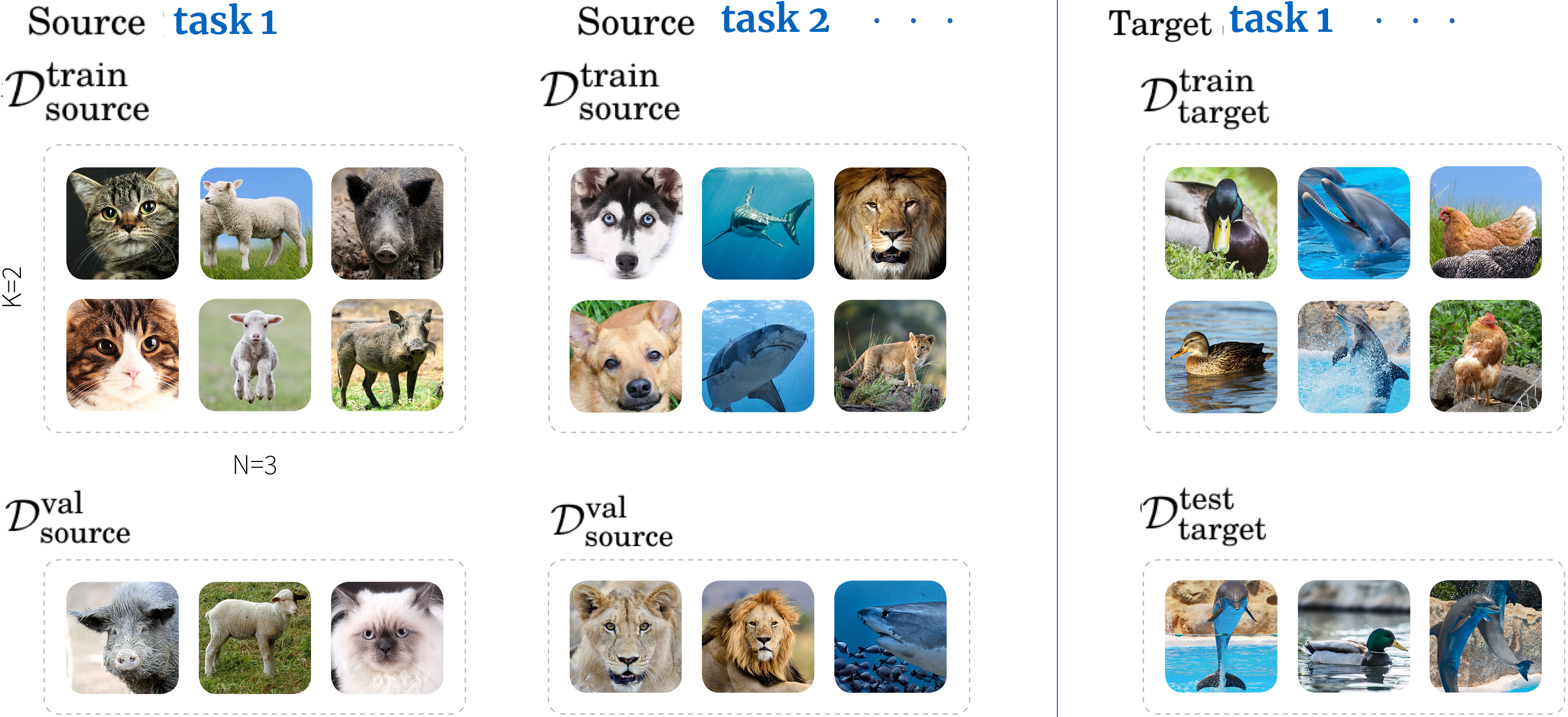
Figure 4: “3-way-2-shot” (few-shot) classification. Each source task’s train set contains 3 classes of 2 examples each (Vinyals et al., 2016). Image modified from Borealis AI blogpost.
MAML: Model-agnostic meta-learning
- MAML finn17_maml is a simple and popular approach of two phases:
- During meta-training (bold line), learn a good weight initialization \(\color{blue}{\omega^*}\) for fine-tuning on target tasks.
- During meta-testing (dashed lines), find the optimal \(\theta^*_i\) for each new task \(i\).
- Good performance
- MAML substantially outperformed other approaches on few-shot image classification (Omniglot, MiniImageNet2), and improved adaptability of RL agent.
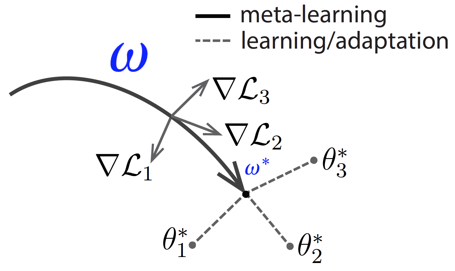
Figure 5: Visualized MAML (image modified from BAIR blogpost).
A little side-note
- Feature reuse, not rapid learning, is the dominant component in MAML.
A little side-note: “Rapid Learning or Feature Reuse? Towards Understanding the Effectiveness of MAML”
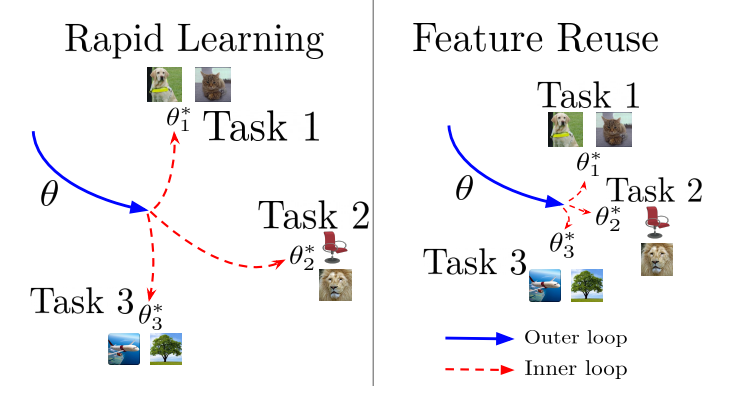
Figure 7: Rapid learning entails efficient but significant change from \(\color{blue}{\omega^*}\) to \(\theta^*\); feature reuse is where \(\color{blue}{\omega^*}\) already provides high quality representations. Figure 1 from the paper.
- Feature reuse, not rapid learning, is the dominant component in MAML.
- Used CCA and CKA to study the learnt representations.
- Led to a simplified algorithm, ANIL, which almost completely removes the inner optimization loop with no reduction in performance.
- Benchmark datasets (e.g. Omniglot, MiniImageNet2) are artifically segmented from the same dataset, hence it might be very easy to reuse features. Interesting to consider less similar tasks (e.g. Meta-dataset, Triantafillou et al. 2019).
Conventional ML: fixed/pre-specified \(\color{blue}{\omega}\)
| Shared meta-knowledge \(\color{blue}{\omega}\) | Task-specific \(\theta\) | |
|---|---|---|
| NN | Hyperparameters (e.g. learning rate, weight initialization scheme, optimizer, architecture design) | Network weights |
Meta-learning: learnt \(\color{blue}{\omega}\) from \(\mathcal{D}_{\mathrm{source}}\)
| Shared meta-knowledge \(\color{blue}{\omega}\) | Task-specific \(\theta\) | |
|---|---|---|
| Hyperopt | Hyperparameters (e.g. learning rate) | Network weights |
| MAML | Network weights (initialization learnt from \(\mathcal{D}_{\mathrm{source}}\)) | Network weights (tuned on \(\mathcal{D}_{\mathrm{target}}\)) |
| NP | Network weights | Aggregated target context [latent] representation |
| Meta-GP | Deep mean/kernel function parameters | None (a GP is fit on \(\mathcal{D}_{\mathrm{target}}^{\mathrm{train}}\)) |
A \(\color{blue}{\omega}\) by any other name
- \(\color{blue}{\omega}\) is shared/task-general parameters that work well across different tasks.
- Examples of parameterized task-general components include a metric space vinyals16_matching_networks, an RNN duan16_rl2, a memory-augmented NN santoro16_meta_learn_memory_augmented.
- Again, meta-knowledge \(\color{blue}{\omega}\) specifies “how to learn” \(\theta\).
- \(\color{blue}{\omega}\) is a starting inductive bias for new tasks from old tasks; equivalent to ‘learning a prior’.
- \(\implies\) There is a loose analogy between any meta-learning approach and hierarchical Bayesian inference griffiths19_doing_more_with_less.
- Bayesian inference generically indicates how a learner should combine data with a prior distribution over hypotheses
- Hierarchical Bayesian inference for meta-learning learns that prior through experience (data from related tasks).
Bayesian meta-learning
- Opens opportunities to griffiths19_doing_more_with_less:
- Translate cognitive science insights, which has focused on hierarchical Bayesian models (HBMs), to ML.
- Use probabilistic generative models from Bayesian deep learning toolbox for meta-learning.
- Useful for safety-critical few-shot learning (e.g. medical imaging), active learning, and exploration in RL (à la Marc Deisenroth’s talk on probabilistic RL).
MAML as a HBM
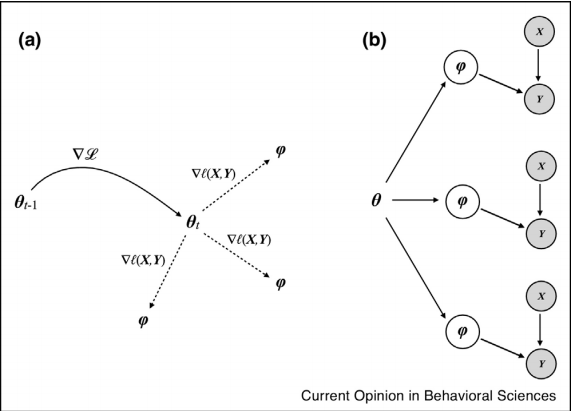
Figure 8: MAML and its corresponding probabilistic graphical model. Figure 2 from Griffiths et al. (2019).
- Grant et al. (2018) grant18_recast_gradient_based_meta_learn show that:
- The few steps of gradient descent by the task-specific learners result in \(\theta^*\), which is an approximation to the Bayesian estimate of \(\theta\) for that task, with a prior that depends on the initial parameterization \(\color{blue}{\omega^*}\) .
- \(\implies\) Learning \(\color{blue}{\omega}\) is equivalent to learning a prior.
LVM + amortized VI for meta-learning
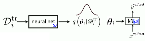
Figure 9: Same at meta-train \(\left(\mathcal{D}_{\text {source}}^{\text {train}}, \mathcal{D}_{\text {source}}^{\text {val}}\right)\) and meta-test \(\left(\mathcal{D}_{\text {target}}^{\text {train}}, \mathcal{D}_{\text {target}}^{\text {test}}\right)\) time.
- Standard VAE optimizes ELBO \(p(\mathbf{x}) \geq \text{ELBO} = \mathbb{E}_{\mathbf{z}\sim q_\phi(\mathbf{z}\vert\mathbf{x})} \left[ \log p_\theta(\mathbf{x}\vert\mathbf{z}) \right] - D_\text{KL}(q_\phi(\mathbf{z}\vert\mathbf{x}) \| p_\theta(\mathbf{z}))\)
- Neural Processes garnelo18_neural_proces, Versa gordon18_meta_learn_probab_infer_predic etc. take inspiration from VAE for meta-learning by treating \(\theta\) as \(\mathbf{z}\).
- \(\log p\left(\mathbf{Y}_{T} \mid \mathbf{X}_{T}, \mathbf{X}_{C}, \mathbf{Y}_{C}\right) \geq \mathbb{E}_{q\left(\mathbf{z} \mid \mathbf{s}_{T}\right)}\left[\log p\left(\mathbf{Y}_{T} \mid \mathbf{X}_{T}, \mathbf{r}_{C}, \mathbf{z}\right)\right] - D_{\mathrm{KL}}\left(q\left(\mathbf{z} \mid \mathbf{s}_{C}, \mathbf{s}_{T}\right) \| q\left(\mathbf{z} \mid \mathbf{s}_{C}\right)\right)\)
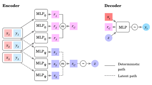
Figure 10: In an NP, meta-parameters \(\color{blue}{\omega}\) are the weights of the encoder and decoder NNs.
GPs for meta-learning
- Use a neural network for the mean or kernel function fortuin19_deep_mean_funct_meta_learn_gauss_proces
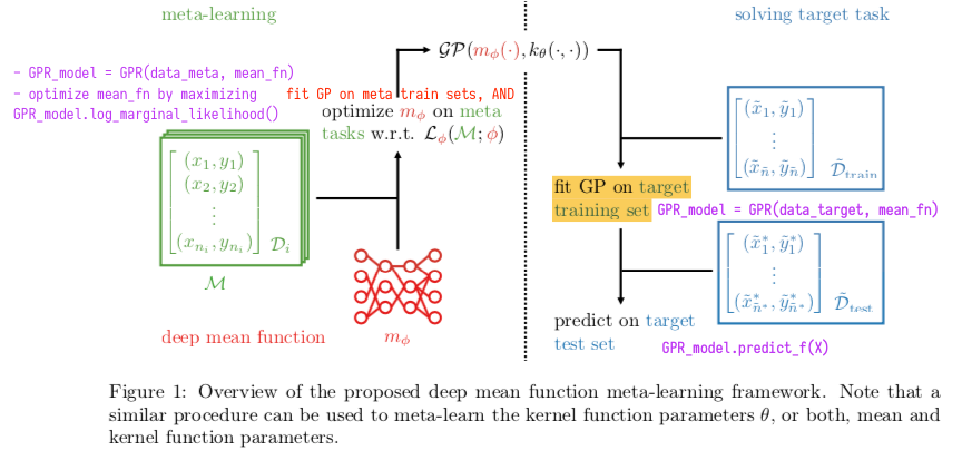
Figure 11: Figure 1 from Fortuin et al. (2019). Corresponding GPFlow code in purple.
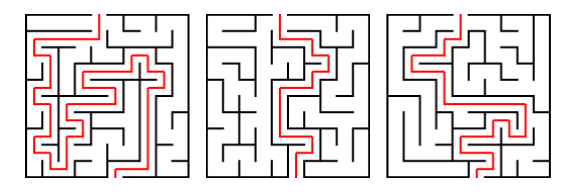
What else can it be used for?
- RL agent trains on some mazes and is tested on unseen mazes generated by the same process duan16_rl2,mishra17_snail_metalearner
Many methods and applications
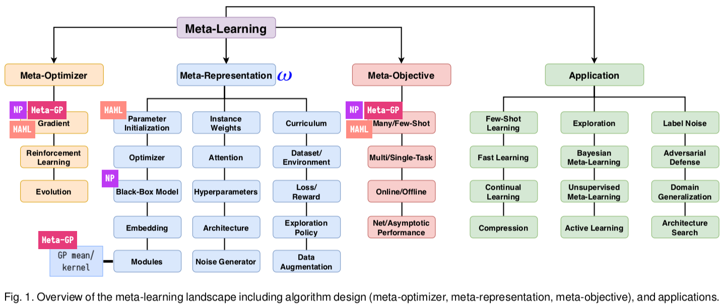
Figure 13: Modified from Figure 1 in Hospedales et al. (2020).
Conclusion
- The core idea of meta-learning is to optimize a model over a distribution of learning tasks \(p(\mathcal{T})\), rather than just a single task, with the goal of generalizing to other tasks from \(p(\mathcal{T})\).
To recap, conventional ML: fixed/pre-specified \(\color{blue}{\omega}\)
| Shared meta-knowledge \(\color{blue}{\omega}\) | Task-specific \(\theta\) | |
|---|---|---|
| NN | Hyperparameters (e.g. learning rate, weight initialization scheme, optimizer, architecture design) | Network weights |
Meta-learning: learnt \(\color{blue}{\omega}\) from \(\mathcal{D}_{\mathrm{source}}\)
| Shared meta-knowledge \(\color{blue}{\omega}\) | Task-specific \(\theta\) | |
|---|---|---|
| Hyperopt | Hyperparameters (e.g. learning rate) | Network weights |
| MAML | Network weights (initialization learnt from \(\mathcal{D}_{\mathrm{source}}\)) | Network weights (tuned on \(\mathcal{D}_{\mathrm{target}}\)) |
| NP | Network weights | Aggregated target context [latent] representation |
| Meta-GP | Deep mean/kernel function parameters | None (a GP is fit on \(\mathcal{D}_{\mathrm{target}}^{\mathrm{train}}\)) |
Bibliography
- [lake16_build_machin_that_learn_think_like_peopl] Lake, Ullman, Tenenbaum, Joshua & Gershman, Building Machines That Learn and Think Like People, CoRR, (2016). link.
- [lake15_human_level_concept_learning] Lake, Salakhutdinov & Tenenbaum, Human-level concept learning through probabilistic program induction, Science, 350, 1332-1338 (2015). doi.
- [hospedales20_meta_learn_neural_networ] Hospedales, Antoniou, , Micaelli & Storkey, Meta-Learning in Neural Networks: a Survey, CoRR, (2020). link.
- [griffiths19_doing_more_with_less] Griffiths, Callaway, Chang, Grant, Krueger & Lieder, Doing more with less: meta-reasoning and meta-learning in humans and machines, Current Opinion in Behavioral Sciences, 29, 24-30 (2019).
- [finn17_maml] Finn, Abbeel & Levine, Model-agnostic meta-learning for fast adaptation of deep networks, 1126-1135, in in: International Conference on Machine Learning (ICML), edited by (2017)
- [vinyals16_matching_networks] Vinyals, Blundell, Lillicrap, Wierstra & others, Matching networks for one shot learning, 3630-3638, in in: Advances in neural information processing systems, edited by (2016)
- [duan16_rl2] Duan, Schulman, Chen, , Bartlett, Sutskever, Abbeel & Pieter, RL$^2$: Fast Reinforcement Learning Via Slow Reinforcement Learning, CoRR, (2016). link.
- [santoro16_meta_learn_memory_augmented] Santoro, Bartunov, Botvinick, Wierstra & Lillicrap, Meta-Learning with Memory-Augmented Neural Networks, 1842-1850, in in: International Conference on Machine Learning (ICML), edited by (2016)
- [grant18_recast_gradient_based_meta_learn] Grant, Finn, Levine, , Darrell & Griffiths, Recasting Gradient-Based Meta-Learning As Hierarchical Bayes, CoRR, (2018). link.
- [garnelo18_neural_proces] Garnelo, Schwarz, Rosenbaum, Dan, Viola, Rezende, , Eslami & Teh, Neural Processes, arXiv preprint: 1807.01622, (2018).
- [gordon18_meta_learn_probab_infer_predic] Jonathan Gordon, John Bronskill, Matthias Bauer, Sebastian Nowozin & Richard Turner, Meta-Learning Probabilistic Inference for Prediction, , (2019). link.
- [fortuin19_deep_mean_funct_meta_learn_gauss_proces] Fortuin & R\"atsch, Deep Mean Functions for Meta-Learning in Gaussian Processes, CoRR, (2019). link.
- [mishra17_snail_metalearner] Mishra, Rohaninejad, Chen & Abbeel, A simple neural attentive meta-learner, in in: Workshop on Meta-Learning, NeurIPS, edited by (2017)