BOLFI
 Available as 🔗 presentation slides or as a 🔗 blogpost.
Problem
- Topic: Statistical inference for models where:
- The likelihood \(p_{\mathbf{y}|\mathbf{\theta}}\) is intractable 🔮 (e.g. analytical form is unknown/costly to compute).
- \(\implies\) inference with likelihood \(\mathcal{L}(\mathbf{\theta}) = p_{\mathbf{y}|\mathbf{\theta}}(\mathbf{y}_o | \mathbf{\theta})\) is not possible.
- Simulating data 🤖 from the model is possible.
- Using a simulator-based statistical model (implicit/generative model), i.e. a family of pdfs \(\left\{p_{\mathbf{y} \mid \mathbf{\theta}} \right\}_{\mathbf{\theta}}\) of unknown analytical form which allows for exact sampling of data \(\mathbf{y} \sim p(\mathbf{y}|\mathbf{\theta})\)
- The likelihood \(p_{\mathbf{y}|\mathbf{\theta}}\) is intractable 🔮 (e.g. analytical form is unknown/costly to compute).
- Inference principle: Find parameter values \(\theta\) for which there is a small distance between
- the posterior of the simulated data \(\mathbf{y}\), and
- the observed data \(\mathbf{y}_o\).
Other assumptions
- Only a small number of parameters are of interest (theta is low-dimensional)
- Data generating process can be very complex
Existing methods
For likelihood-free inference with simulator-based models, the basic idea is to identify model parameters by finding values which yield simulated data that resemble the observed data.
- “Approximate Bayesian computation” (ABC), originated in genetics 🔬
- “Indirect inference”, originated in economics 📈
- “Synthetic likelihood”, originated in ecology 🌲
Conventional ABC
- “Bayesian forward modeling”, i.e. likelihood-free rejection sampling (LFRS)
- Let \(\mathbf{y}_o\) be the observed data. For many iterations:
- Sample \(\theta\) from proposal distribution \(q(\theta)\).
- Sample \(\mathbf{y}|\theta\) according to the data model.
- Compute distance \(d(\mathbf{y}, \mathbf{y}_o)\)
- Keep if \(d(\mathbf{y}, \mathbf{y}_o) \leq \epsilon\); discard otherwise.
- Different \(q(\theta)\) for different algorithms
- If \(\epsilon\) is small enough, kept samples are samples from an approximate posterior
Implicit likelihood approximation
- Compute likelihood (probability of generating data like \(\mathbf{y}_o\) given hypothesis \(\theta\)) empirically
- Proportion of kept (green) samples
- \(L(\theta) \approx \frac{1}{N} \sum_{i=1}^{N} \mathbb{1}\left(d\left(y_{o}^{(i)}, y^{\circ}\right) \leq \epsilon\right)\)
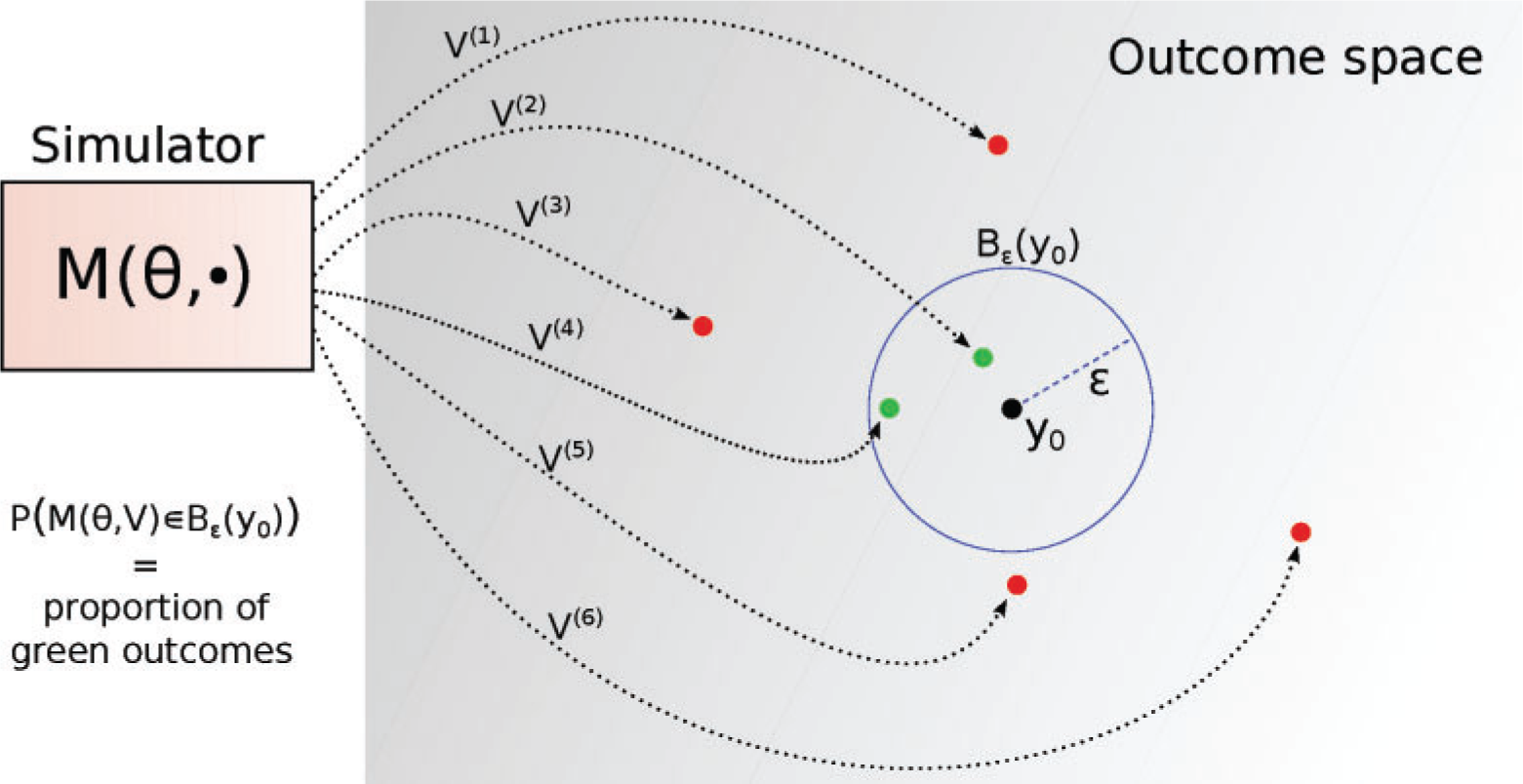 Image from 10.1093/sysbio/syw077
Downsides
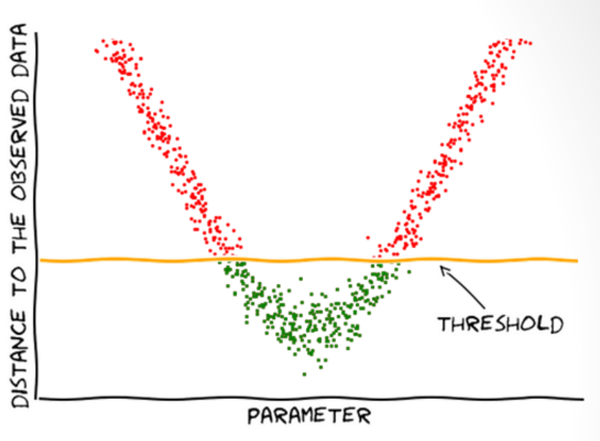 Image from Leclerq:online
\(L(\theta) \approx \frac{1}{N} \sum_{i=1}^{N} \mathbb{1}\left(d\left(y_{o}^{(i)}, y^{\circ}\right) \leq \epsilon\right)\)
Image from Leclerq:online
\(L(\theta) \approx \frac{1}{N} \sum_{i=1}^{N} \mathbb{1}\left(d\left(y_{o}^{(i)}, y^{\circ}\right) \leq \epsilon\right)\)
- Rejects most samples when \(\epsilon\) is small
Does not make assumptions about the shape of \(L(\theta)\)
Does not use all information available.
Aims at equal accuracy for all parameters
BOLFI
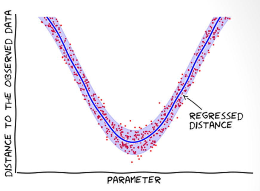 Image from Leclerq:online
- Does not reject samples; learns from them (i.e. builds a statistical model of the distances w.r.t. the parameters).
- Models the distances, assuming the average distance is smooth.
- Use Bayes’ theorem to update the proposal of new points.
- Prioritize parameter regions with small distances.
Regressing effective likelihood
- Data are tuples \((\theta_i, d_i)\), where \(d_i = d(\mathbf{y}_\theta^{(i)}, \mathbf{y}_o)\)
- Model conditional distribution \(d \mid \theta\)
Approximate likelihood function for some choice of \(\epsilon\):
- \(\hat{L}(\theta) \propto \hat{P}(d\leq \epsilon \mid \theta)\)
- Choice of \(\epsilon\) is delayed until the end, after the learning of the model.
Regressing effective likelihood
- Fit a log Gaussian process (GP) to regress how the parameters affect the distances and use Bayesian optimization.
- Squared exponential covariance function
- Log transform because distances are non-negative
- Approach is not restricted to GPs
Data acquisition
- Use Bayesian optimization to prioritize regions of \(\theta\) where \(d\) tends to be small.
- Sample \(\theta\) from an adaptively constructed proposal distribution, e.g. the lower confidence bound acquisition function.
- \(\mathcal{A}_{t}(\theta)=\underbrace{\mu_{t}(\theta)}_{\text {post mean }}-\sqrt{\underbrace{\eta_{t}^{2}}_{\text {weight }} \underbrace{v_t(\theta)}_{\text {post var }}}\), \(t\): no. of samples acquired
- “We used the simple heuristic that \(\theta_{t+1}\) is sampled from a Gaussian with diagonal covariance and mean equal to the minimizer of the acquisition function. The standard deviations were determined by finding the end-points of the interval where the acquisition function was within a certain (relative) tolerance.”
- Approach is not restricted to this acquisition function.
Bayesian optimization in action
 Image from Leclerq:online
Close the loop
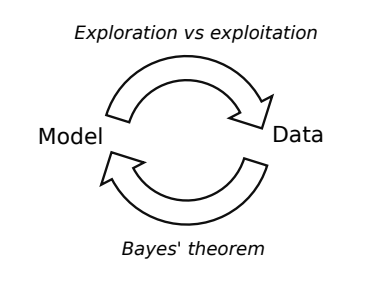 Image from 10.1093/sysbio/syw077
- Exploration: where the uncertainty is high
- Exploitation: where posterior mean is smallest
- Use Bayes’ theorem to update the model in light of new data
- As opposed to usual applications of Bayesian optimization, here the objective function is highly stochastic.
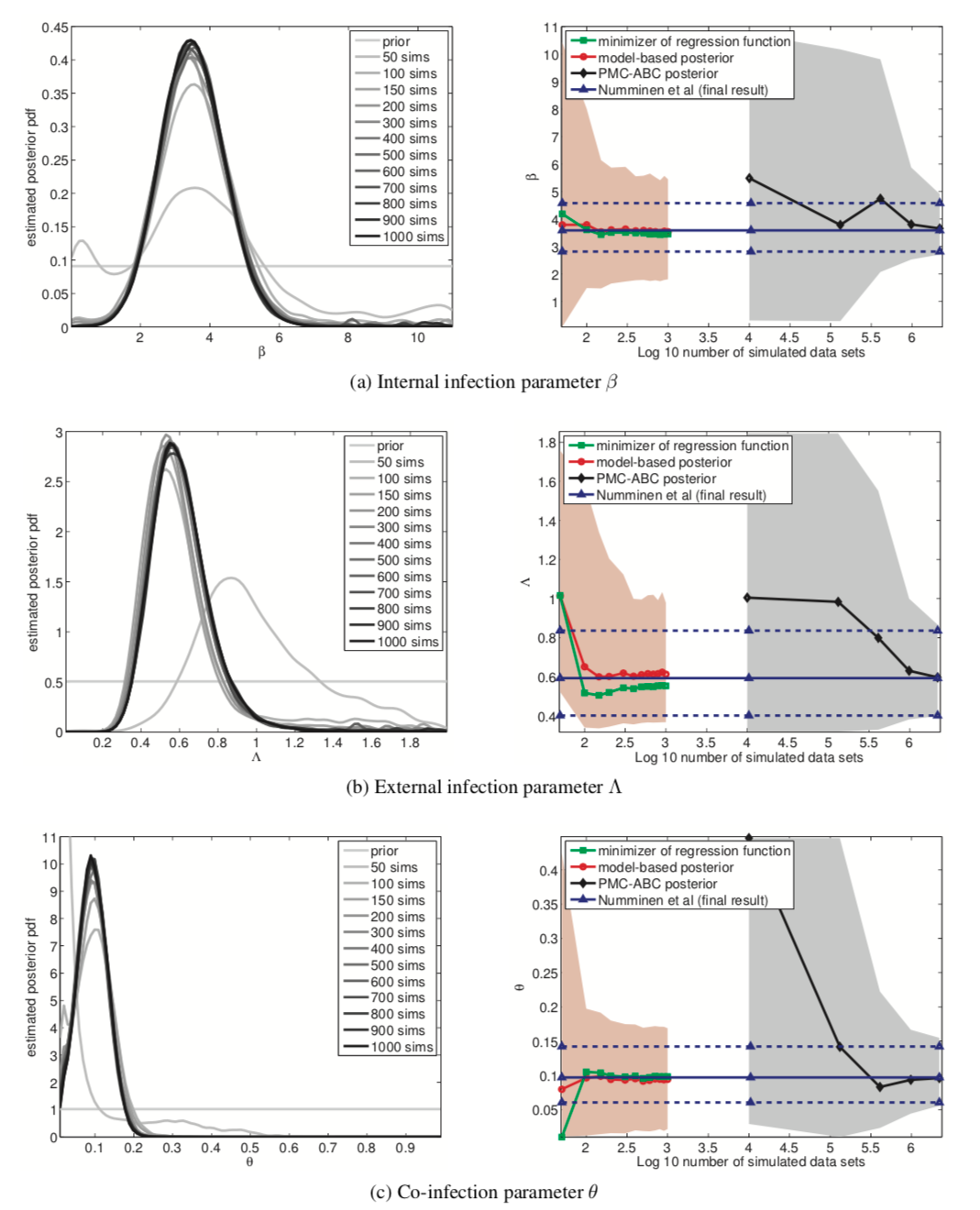
Results
- Roughly equal results with 1000x fewer simulations
- Monte Carlo ABC: 4.5 days with 300 cores
- BOLFI: 90 minutes with seven cores
- Data of bacterial infections in child care centers.
- Data generating process is defined via a latent continuous-time Markov chain and an observation model.
- “Developed by Numminen et a.l (2013) to infer transmission dynamics of bacterial infections in day care centers.”
Figure 12
Advantages
- Inference more efficient, far more comprehensive data analysis.
- Enables inference for e.g. models of evolution where simulating a single data set takes 12-24 hours.
- Enables investigation of model identifiability, or the influence of distance measure on likelihood function.
- We get an explicit construction of an approximate likelihood function, whereas with conventional ABC only had an implicit likelihood function.
Further research
- Distance measures
- Acquisition function
- Efficient high-dimensional inference
- Use this advantage from Bayesian optimization
Conclusion
BOLFI combines …
- Statistical modeling (GP regression) of the distance between observed and simulated data
- Decision making under uncertainty (Bayesian optimization).
…to increase efficiency of inference by several orders of magnitude.
Links and reference Practical
Bibliography
Bibliography
- [10.1093/sysbio/syw077] Lintusaari, Gutmann, Dutta, Kaski & Corander, Fundamentals and Recent Developments in Approximate Bayesian Computation, Systematic Biology, 66(1), e66-e82 (2016). link. doi.
- [Leclerq:online] @miscLeclerq:online, author = Florent Leclercq, title = Bayesian optimisation for likelihood-free cosmological inference, howpublished = \urlhttp://www.florent-leclercq.eu/talks/2018-10-22_IHP.pdf, month = , year = , note = (Accessed on 11/03/2019. Recording at https://www.youtube.com/watch?v=orDbPZFd7Gk&t=41s.)