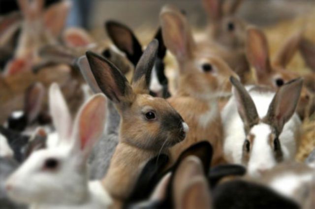
Neural Ordinary Differential Equations 🐰🦊
Presented by Christabella Irwanto
Neural ODE
- A new model class chen18_neural_ode, can be used as
- Continuous-depth residual networks
- Continuous-time latent variable models
- Propose continuous normalizing flows, generative model
- Scalable backpropagation through ODE solver
- Paper shows various proofs of concept
ODE? 😕
“In the 300 years since Newton, mankind has come to realize that the laws of physics are always expressed in the language of differential equations.”
- Steven Strogatz
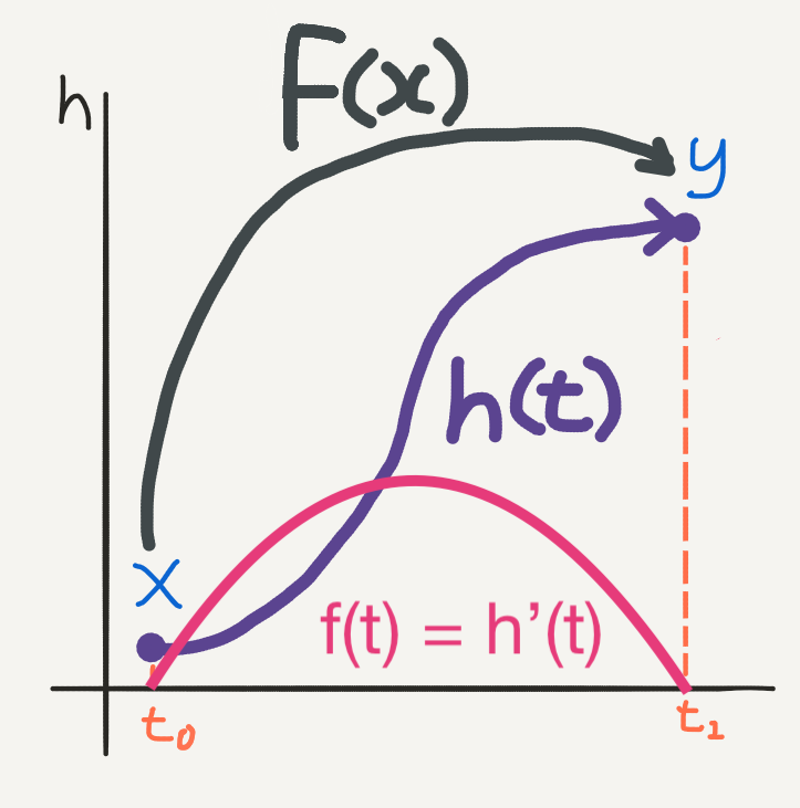
- An ODE is an equation involving an unknown function \(y=f(t)\) and at least one of its derivatives \(y’, y''\) etc.
- Univariate functions (“time”) vs partial DE’s with multivariate input
- Solve ODE by finding satisfying function \(f\)
- Useful whenever it’s easier to describe change than absolute quantity, e.g. in many dynamical systems (☢, 🏀, 💊)
Bunny example 🐇
- Model system of dynamics with first-order ODE, \(B'(t) = \frac{dB}{dt} = rB\)
- \(B(t)\): bunny population at time \(t\)
- \(r\): growth rate of new bunnies for every bunny, per \(\Delta t\)
Visualize ODE
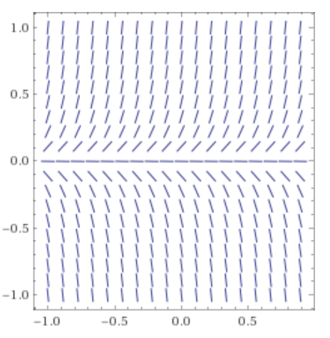
Slope field of derivative for each \((B, t)\)
Solve ODE
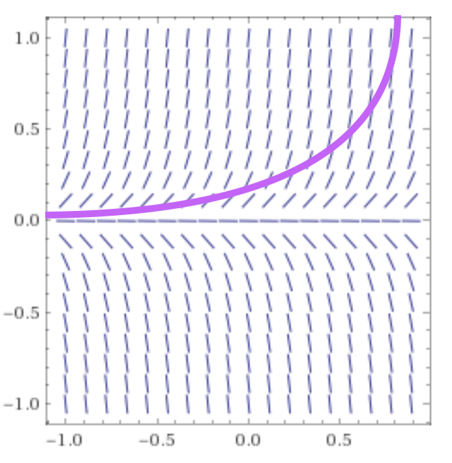
- Analytical solution via integration is \(B(t) = B(t_0)e^{rt}\)
- Known initial value \(B(t_0)\)
Numerical ODE solver
- Not all ODE’s have a closed form function satisfying it
- Even if so, it’s very hard finding solutions
- We have to numerically solve the ODE
- Euler’s method, Runge-Kutta methods
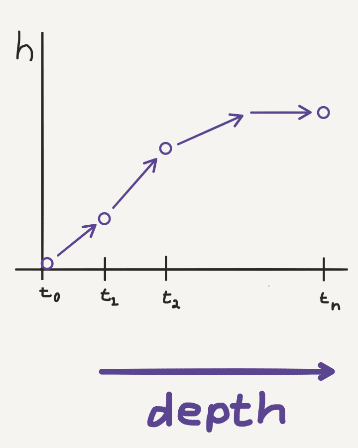
Enter neural networks
- Regular neural networks transform input with a series of functions \(f\),
\(\mathbf{h}_{t+1} = f(\mathbf{h}_t)\)
- Each layer introduces error that compounds
- Mitigate this by adding more layers, and limit the complexity of each step
- Infinite layers, with infinitesimal step-changes?
Resnet
- Instead of \(\mathbf{h}_{t+1} = f(\mathbf{h}_t)\), learn \(\mathbf{h}_{t+1} = \mathbf{h}_t + f(\mathbf{h}_t, \theta_t)\)
- Similarly, RNN decoders and normalizing flows build complicated transformations by chaining sequences
- Looks like Euler discretization of continuous transformation
Neural ODE
- \(\mathbf{h}_{t+1} = \mathbf{h}_t + f(\mathbf{h}_t, \theta_t)\)
- In the continuous limit w.r.t. depth \(t\), parameterize hidden state dynamics with an ODE specified by a neural network:
- \(\frac{d\mathbf{h}(t)}{dt} = f(\mathbf{h}(t), t, \theta)\), where neural network \(f\) has parameters \(\theta\)
- Function approximation now over a continuous hidden state dynamic
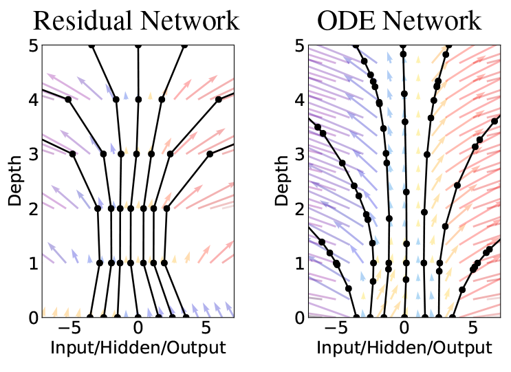
Resnet vs neural ODE
Forward pass
- 🐰 Evaluate \(\mathbf{h}(t_1)\) by solving the integral
- \(\mathbf{h}(t) = \int f(t, \mathbf{h}(t), \theta_t)dt\)
- If we use Euler’s method, we get exactly the residual state update!
Numerical ODE solver
- Paper solves ODE initial value problems numerically with implicit Adams method
- Not unconditionally stable
- Current set of PyTorch ODE solvers only applicable to (some) non-stiff ODEs
- Without a reversible integrator (implicit Adams is not reversible), method drifts from the true solution doing a backwards integration
Advantages
- Use existing efficient solvers to integrate neural network dynamics
- Memory cost is \(O(1)\) due to reversibility of ODE net
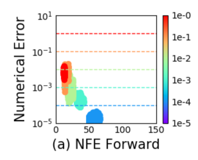
- Tuning ODE solver tolerance gives trade-off between accuracy and speed
- More fine-grained tuning,versus using lower precision floating point numbers
Backward pass
- Output (hidden state at final depth) is used to compute loss
\begin{equation}
L(\mathbf{z}(t_1)) = L\left( \mathbf{z}(t_0) + \int_{t_0}^{t_1}
f(\mathbf{z}(t), t, \theta)dt \right) =
L(\textrm{ODESolve}(\mathbf{z}(t_0), f, t_0, t_1, \theta))
\end{equation}
- Scalable backpropagation through ODE solver with adjoint method
- Vectorization to compute multiple derivatives in single call
How to train?
- Standard reverse mode chain rule equations in backprop
- Take continuous time limit of chain rule to recover the adjoint sensitivity equations
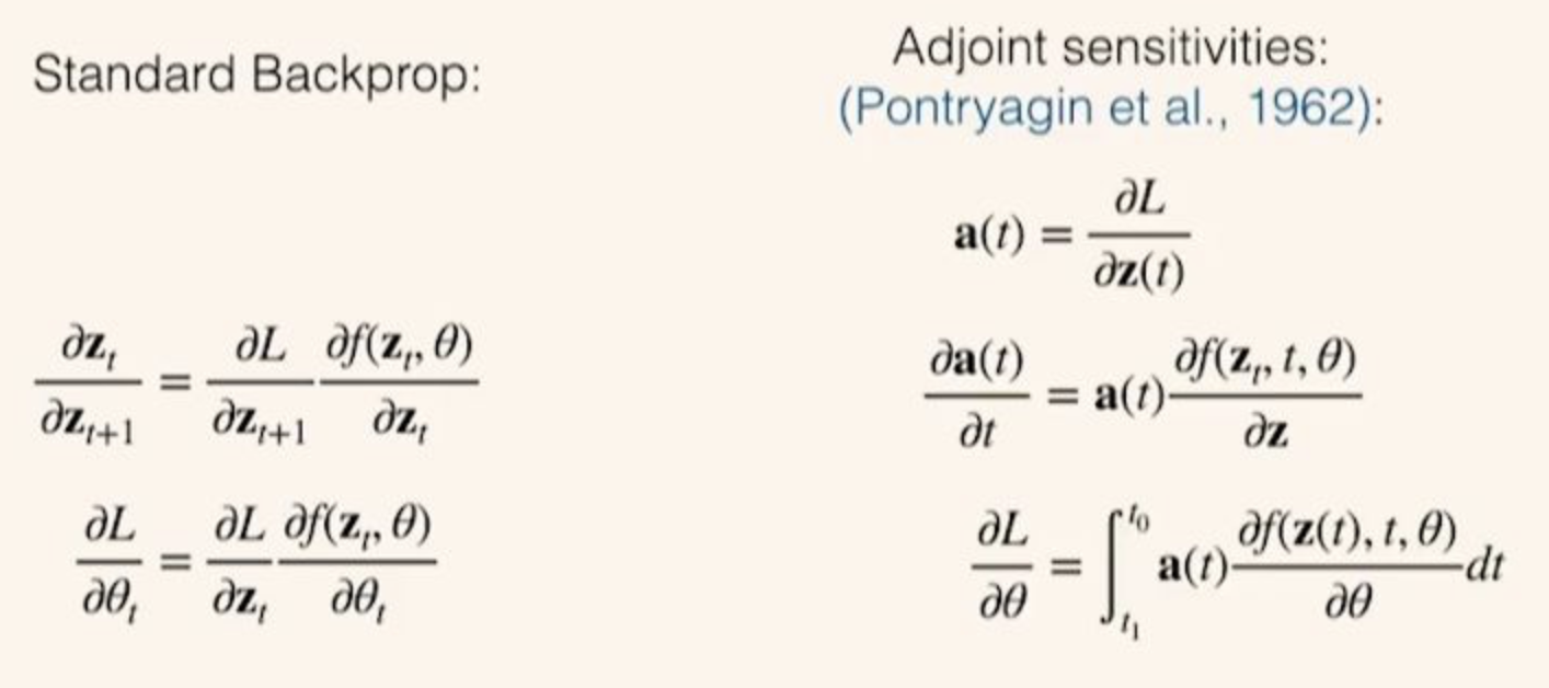
Adjoint sensitivity
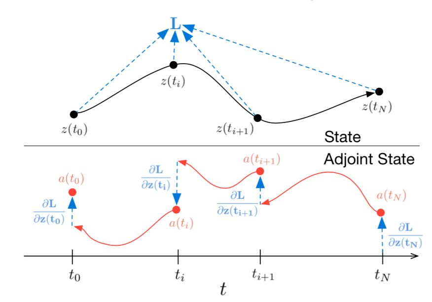
- Reverse-mode differentiation of an ODE solution
- Solving for adjoint state with same ODE solver used in forward pass
Results of ODE-Net vs Resnet
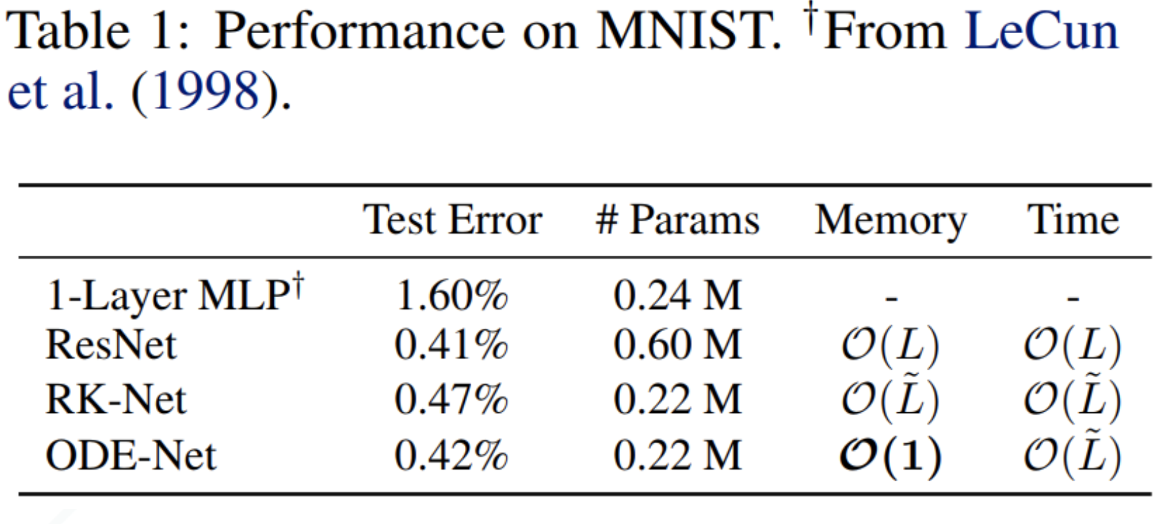
- Fewer parameters with same accuracy
- However, harder to train, tricky to implement mini-batching
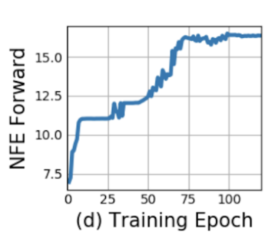
- Can't control the training time cost, computational complexity increases
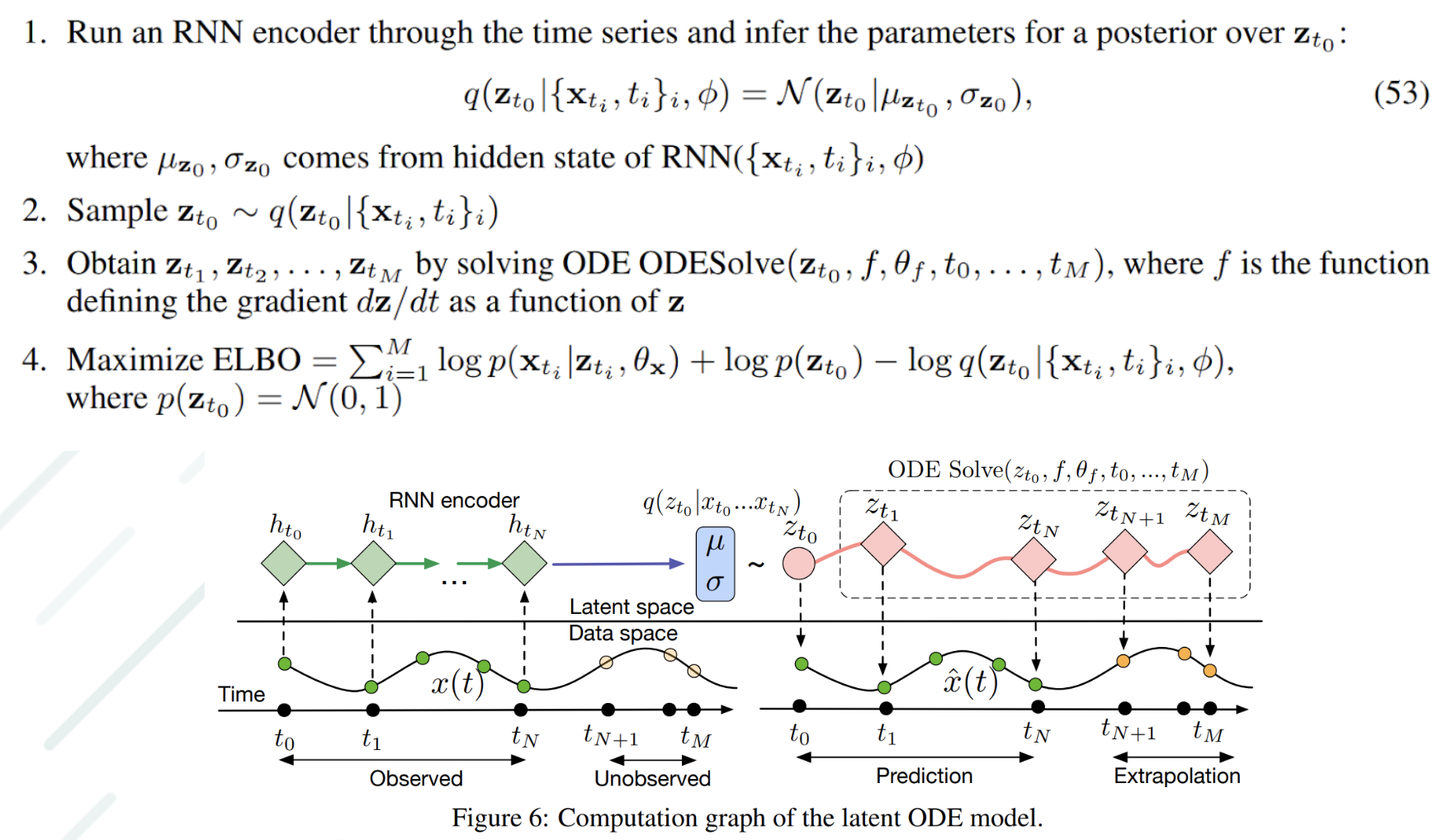
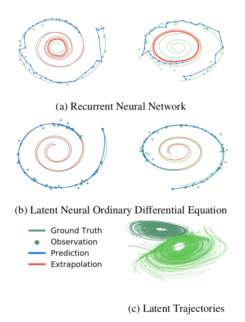
Generative latent time-series model
- Continuous-time approach to modeling time series
Results of experiments
- Spiral dataset at irregular time intervals, with Gaussian noise
Advantages
- For supervised learning, its main benefit is extra flexibility in the speed/precision tradeoff.
- For time-series problems, allow handling of data at irregular intervals
Normalizing flows
- Normalizing flows define a parametric density by iteratively transforming Gaussian sample:
\begin{align}
z_0 &\sim Normal(0, I) \\
z_1 &= f_0(z_0) \\
… \\
x &= f_t(z_t)
\end{align}
- Use the change of variables formula to compute p(x): \(log p(z_{t+1}) = log p(z_t) - log | det \frac{df(z_t)}{dz_t} |\)
- Paper proposes continuous-time version, Continuous NF
- Derived continuous-time analogue of change of variables formula:
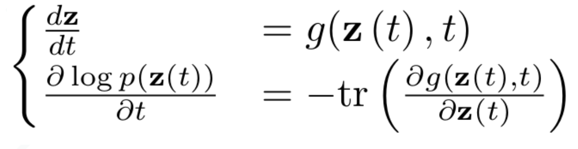
Results
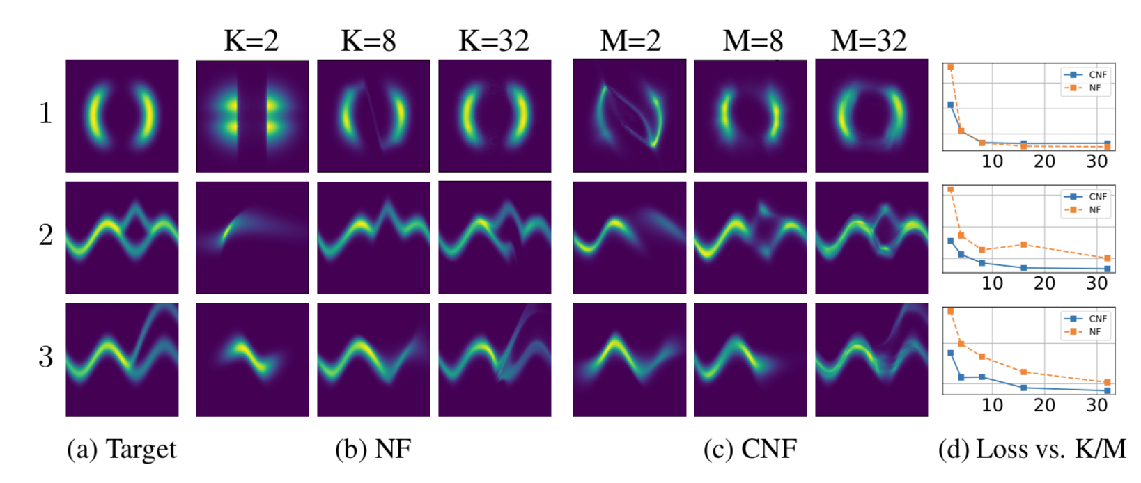
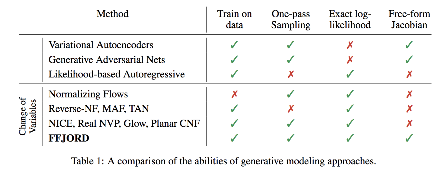
- Compare Continuous NF to NF family of models on density estimation, image generation, and variational inference
- Achieve state-of-the-art among exact likelihood methods with efficient sampling, in follow-up paper grathwohl18
Pros and cons
- 4-5x slower than other methods (Glow, Real-NVP)
Summary
- New and novel application of differential equation solvers as part of a neural net
- Idea of Resnet/RNN as an Euler discretization is a neat solution
- Much work can be done on both numerical differential equation and ML side
References
Code:
- https://nbviewer.jupyter.org/github/urtrial/neural_ode/blob/master/Neural ODEs.ipynb
- https://github.com/kmkolasinski/deep-learning-notes/tree/master/seminars/2019-03-Neural-Ordinary-Differential-Equations (ODE solver implementations etc.), companion to very awesome slides including adjoint method derivations
Blogposts
- https://jontysinai.github.io/jekyll/update/2019/01/18/understanding-neural-odes.html
- https://blog.acolyer.org/2019/01/09/neural-ordinary-differential-equations/
- https://braindump.jethro.dev/posts/neural_ode/
- https://towardsdatascience.com/neural-odes-breakdown-of-another-deep-learning-breakthrough-3e78c7213795
- https://towardsdatascience.com/paper-summary-neural-ordinary-differential-equations-37c4e52df128
For adjoint sensitivity:
Original content from author(s)
Bibliography
- [chen18_neural_ode] Ricky Chen, Yulia Rubanova, Jesse, Bettencourt & David Duvenaud, Neural Ordinary Differential Equations, , (2018).
- [grathwohl18] Will Grathwohl, Ricky Chen, Jesse Bettencourt, Ilya Sutskever & David Duvenaud, FFJORD: Free-form Continuous Dynamics for Scalable Reversible Generative Models, , (2018).