scikit-learn in a nutshell 🥜

14 Nov 2018

Presented by Christabella Irwanto

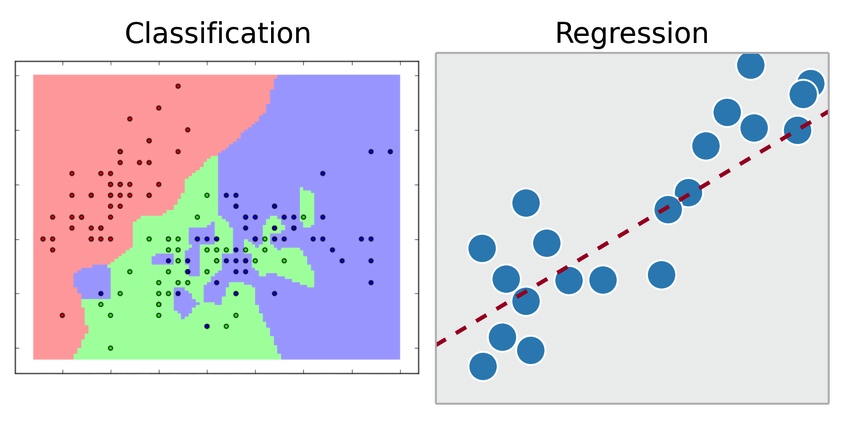
Machine learning?

“Learn” from known data and generalize to unknown data

• Classification predicts a discrete label given input \(x\), e.g. kNN
• Regression predicts a continuous value given \(x\), e.g. linear regression

What about scikit-learn?

• Collection of tools for machine learning in Python
• Built on NumPy and SciPy (scientific computing)

Input data matrix

• data is expected to be “array-like” (e.g. 2-d np.array) or scipy.sparse matrix
• shape of [n_samples, n_features]
  • n_samples: no. of items, e.g. documents/images/rows in a CSV
  • n_features: no. of traits describing each item
• high dimensional data of mostly zero-valued features \(\implies\) scipy.sparse matrices are more memory-efficient

Datasets

• Easily load and fetch datasets
  • Toy (small) datasets 👶 e.g. Boston house prices, Iris plants, handwritten digits, …
  • Real world datasets 💼 e.g. Olivetti faces, 20 newsgroups text documents, …
  • Artificial datasets, e.g. make_moons, make_blobs, make_swiss_roll 🍥

Swiss roll

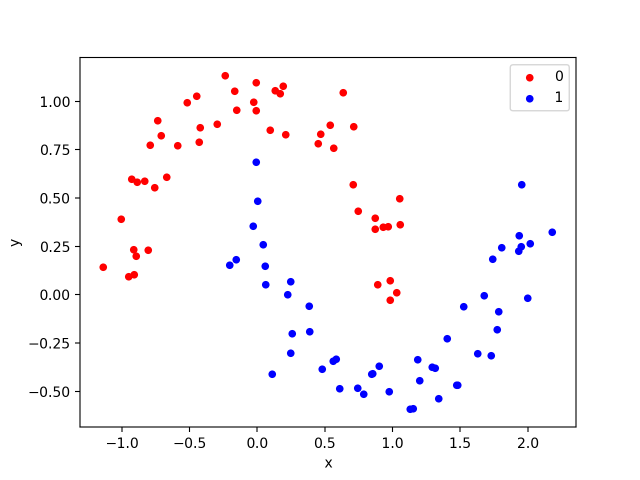
from sklearn import datasets
X, y = datasets.make_moons(n_samples=100, noise=.1)

Feature scaling

• Some algorithms are sensitive to feature scaling (e.g. linear models) while some are not (e.g. decision trees)

• Depending on the data, different scaling methods will be more appropriate.

  • StandardScaler, RobustScaler, MinMaxScaler

  from sklearn.preprocessing import MinMaxScaler
  scaler = MinMaxScaler()
  scaler = scaler.fit(X_train)
  

Feature extraction

• CountVectorizer computes the count of each word.

import pandas as pd
from sklearn.feature_extraction.text import CountVectorizer
>>> corpus = ['Roses are red.',
...           'Violets are red too.']
>>> vectorizer = CountVectorizer();
>>> X = vectorizer.fit_transform(corpus);
>>> pd.DataFrame(X.toarray(),
		 columns=vectorizer.get_feature_names())
   are  red  roses  too  violets
0    1    1      1    0        0
1    1    1      0    1        1

• In information retrieval or text mining, frequency-inverse document frequency (tf-idf) is a popular measure of a word’s importance in a document.

Feature selection

• Most models have in-built feature selection, e.g. feature importance in decision trees
• Can also be done separately with feature_selection module
  • E.g. feature_selection.RFECV
    • Find the best possible subset evaluated with cross-validation
• Also SelectKBest, SelectFromModel

Hyperparameter optimization

• Manually iterate through parameter values, or…
• sklearn.grid_search.GridSearchCV, RandomizedGridSearchCV

from sklearn.linear_model import Ridge, RidgeCV
from sklearn.grid_search import GridSearchCV
model = Ridge()
gs = GridSearchCV(model, {alpha=[0.01, 0.05, 0.1]}, cv=3).fit(X, y)
gs.best_params

• Some models have versions with built-in cross-validation; more efficient on large datasets

model = Ridge(alphas=[0.01, 0.05, 0.1], cv=3).fit(X, y)
model.alpha_  # Best alpha

Dimensionality reduction

• PCA: deterministic, inductive (learns a model that can be applied to unseen data)
• TSNE: stochastic, transductive (models data directly)
• SparseRandomProjection: more memory efficient, faster computation

Model selection

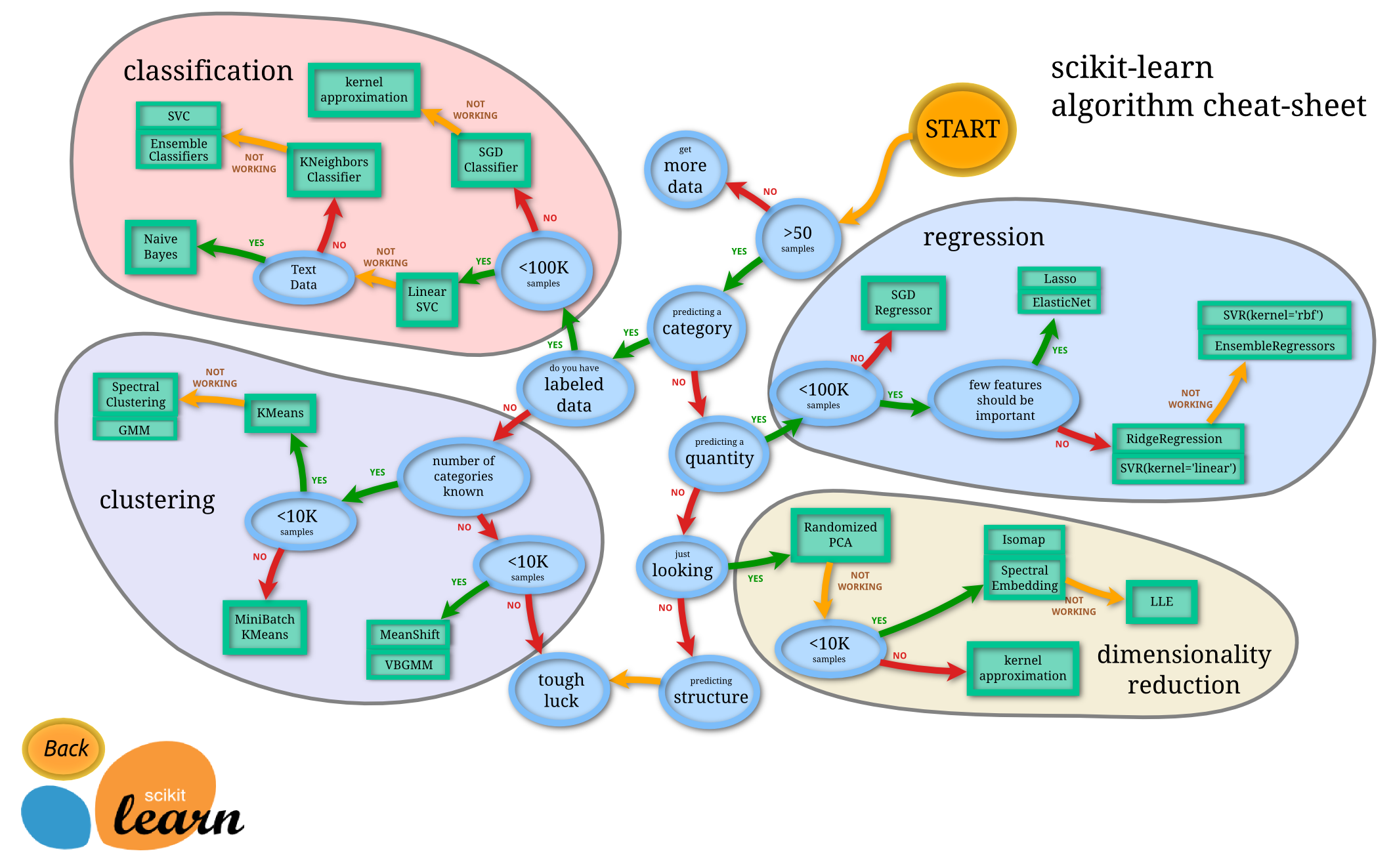
All the ML algorithms

Find them (and more) in the User Guide!

• Regression vs classification
• Parametric: assumes the forms of the function (mapping data \(X\) to output \(Y\))
  • good: simpler, faster, requires less data
  • bad: common parametric forms rarely fit the underlying densities actually encountered in practice
  • E.g. logistic regression, naive bayes, neural networks
• Nonparametric: does not assume the functional form
  • good: flexible, does not require prior knowledge of underlying distribution, can be used with arbitrary distributions
  • bad: needs more training data, slower
  • E.g. kNN, decision tree, SVM

All the ML algorithms

• Supervised: Requires labeled training data
  • E.g. regression, classification
• Unsupervised: On unlabeled data
  • E.g. Clustering, representation learning
    • k-means, principal component analysis, autoencoders, DBSCAN

API’s of sklearn objects

• Estimator: Most important object in sklearn, provides a consistent interface for every machine learning algorithm

  estimator.fit(data[, targets])
  

• Predictor: An estimator supporting predict and sometimes predict_proba, e.g. classifier, regressor, clusterer
  • Also score to judge quality of the fit/prediction on new data
  • Other useful attributes: coef_ (estimated model parameters)
• Transformer: Estimator supporting transform
  • preprocessing, unsupervised dimensionality reduction, kernel approximation, feature extraction

All other modules support the estimator, e.g. datasets, metrics, feature_selection, model_selection, ensemble…

Using the Estimator API

1. Choose and instantiate an estimator
2. Fit the estimator to your data matrix
3. transform data, or predict on test data

The power of estimators

• Many other projects compatible with scikit-learn API conventions
• Meta-estimator: An estimator which takes another estimator as a parameter.
  • E.g. pipeline.Pipeline, model_selection.GridSearchCV, feature_selection.SelectFromModel, ensemble.BaggingClassifier

Pipelines: It’s like Lego

• Plug output of preprocessing PCA into input of SVM classifier: a common pattern
• Pipeline object for chaining estimators, FeatureUnion for estimators in parallel

from sklearn.pipeline import Pipeline
clf = Pipeline([('pca', decomposition.PCA(n_components=150)),
		('svm', svm.LinearSVC(C=1.0))])

clf.fit(X_train, y_train)

y_pred = clf.predict(X_test)

Ensembles

Aggregate the individual predictions of multiple predictors

ensemble_clf = VotingClassifier(estimators=[
			    ('dummy', dummy_classifier),
			    ('logistic', lr),
			    ('rf', RandomForestClassifier())],
			    voting='soft');
ensemble_clf.fit(X_train, y_train);
ensemble_clf_accuracy_ = cost_accuracy(y_test,
   ensemble_clf.predict(X_test));

Metrics

• Measure predictive performance
• metrics.confusion_matrix, metrics.classification_report (combines metrics.f1_score etc.)

>> from sklearn import metrics
>> print(metrics.classification_report(y, y_pred))
	      precision    recall  f1-score   support

     class 0       0.50      1.00      0.67         1
     class 1       0.00      0.00      0.00         1
     class 2       1.00      0.67      0.80         3

weighted avg       0.70      0.60      0.61         5

Splitting data

• Measuring error on training set (used to learn the model’s parameters) is not a good measure of predictive performance
• Evaluate fitted model on a held-out test set

from sklearn import model_selection
X_train, X_test, y_train, y_test = model_selection.train_test_split(X, y,
					test_size=0.25, random_state=0)

• However, this reduces your training data

Cross validation

• Repeatedly split the data into train-test pairs–“folds”

from sklearn.model_selection import cross_val_score
cross_val_score(estimator, X, y, cv=5)  # 5 folds

Assumes that each observation is independent.

Case study

Music genre classification 🌚

github.com/christabella/music-genre-classification/

End-to-end ML workflow:

1. Automated model selection with TPOT
2. Preprocessing
3. Visualizations
4. Splitting
5. Multiple models, using same fit
6. GridSearchCV
7. Ensemble (VotingClassifier)

Optimizing performance

• Scaling to bigger data
• No GPU support
• n_jobs parameter in most estimators to specify number of subprocesses

Conclusion

• Essential tools and classic machine learning algorithms
• Not meant to be…
  • A deep learning package (TensorFlow/PyTorch)
  • A visualization library (matplotlib, seaborn, plotly)
  • A natural language processing toolkit (NLTK, gensim)
  • For basic statistical modeling (statsmodels, SciPy)

Resources

• Glossary of sk-learn terms and API's
• Scikit-learn tutorial